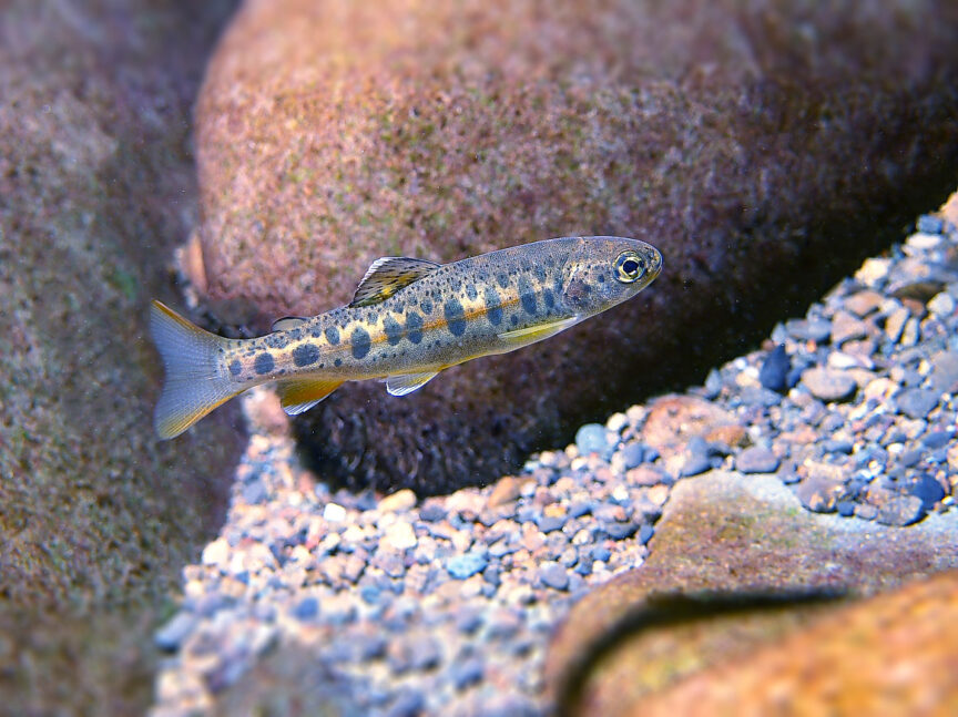
By Nick Chambers
We are back with Part 2 of our installment by Nick Chambers — born and raised in Oregon and former staff for Wild Steelheaders United — on why a catch and release only policy for wild steelhead is the best management alternative for the long-term health and resilience of wild steelhead populations in the southern Oregon coastal region.
Last week, Nick introduced the concept of density dependence, and how assumptions about density dependence are often used to develop escapement goals, which are a critical component of fisheries management. This week, Nick provides a more in depth discussion on the intricacies and quirks of density dependence, why adult spawning distribution is a key consideration, and how those attributes are important to evaluating density dependence and estimating escapement goals.
Let’s start by reviewing the terminology from last week’s post.
Escapement refers to the number of fish that escape the fishery and survive to spawn. An escapement goal is an estimate of how many spawning adults are required to take advantage of the available habitat. Goals that are too low may depress a population beyond its ability to recover, while goals that are too high may be unrealistic and eliminate potential for any fisheries. Ideally, there is a conservation and angling sweet spot that balances the needs of the population to remain resilient to climate change and creates opportunities for anglers to enjoy fishing for wild steelhead.
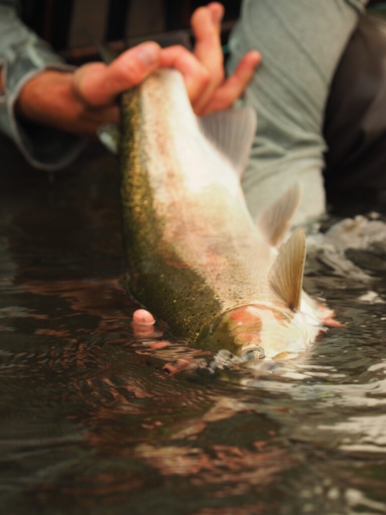
Above image: Nick Chambers
Most methods of estimating escapement goals are based on a population’s ability to compensate for a reduced number of spawning adults, which is where density dependence comes in. Density dependence is how population vital rates, like growth and survival, change in relation to the number of competitors. For example, high densities of juvenile steelhead can result in reduced growth and lower survival if the requirements of the fish exceed the capacity of the habitat.
On the other hand, reducing the number of adults, and in turn, reducing the number of juveniles, can induce a compensatory response. For instance, reduced density of competitors, at least up to a point, may allow juveniles to compensate with increased growth and survival.
Evaluating the effects of density dependence is not easy without high quality data, and systematic, consistent sampling over a sufficient period of time is expensive. For populations of steelhead that are not listed under the Endangered Species Act, like those in Southern Oregon, there is far less available funding for monitoring, which means they are often less studied than populations considered more at-risk.
As noted previously, less data leads to greater assumptions (and more potential adverse impacts to populations from too much angling impact), which is why we are taking a deep dive into the early-life of juvenile salmonids to highlight how effects of density dependence on young-of-the-year fish (YOY) can be conflated with the distribution of spawning adults, potentially leading to erroneous assumptions about capacity.
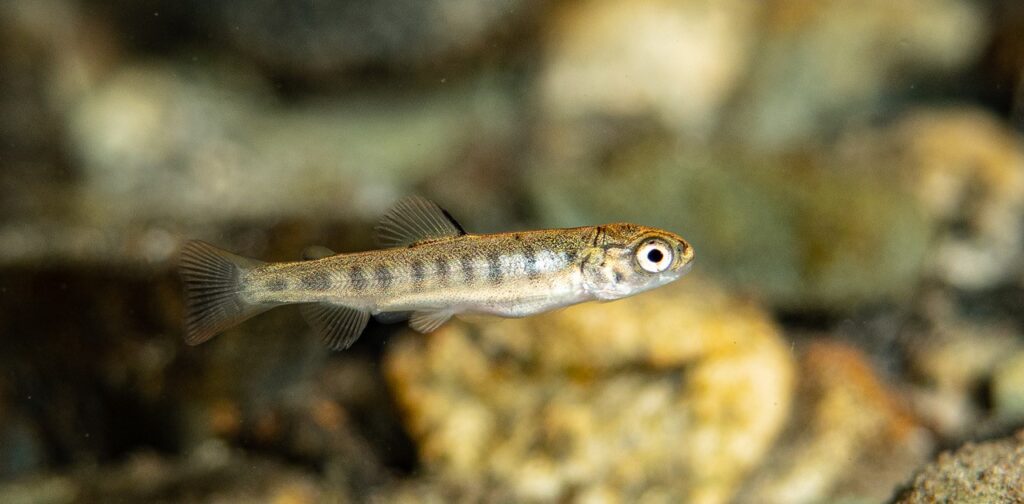
Image: Nick Chambers
Specifically, let’s look at the interaction between adult spawner distribution and early-life density dependence and mortality, and its relevance to evaluating capacity and estimating escapement goals.
Female salmon and steelhead have a lot of eggs, and for good reason — their offspring can and often do experience very high levels of mortality. A female steelhead may carry between 3,000 – 8,000 eggs, depending on stock, age and size, and whether it is a repeat spawner. Generally, steelhead deposit those eggs in the gravel from late winter through spring, and the resulting juveniles will emerge several weeks later, depending on the water temperature.
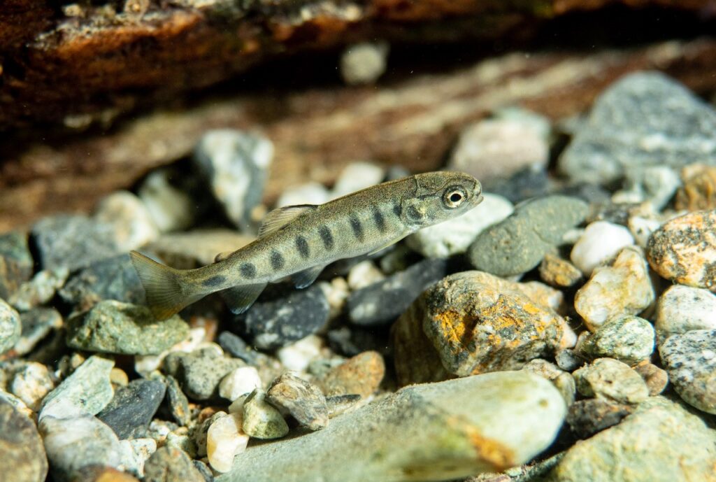
Image: Nick Chambers
After absorbing their yolk sac, the small fish are referred to as fry. Upon emergence, fry are barely an inch long. They are relatively poor swimmers, and as a result, most individuals remain fairly close to the redd during their first summer of life.
In salmonids, the highest mortality rate often occurs within the first two to three months after emergence, when large schools of vulnerable fry compete for food in a very limited space. This is what is commonly referred to as the critical period. This is an apt description because the mortality rates are quite high, and owing to the potentially large numbers of fry, even small changes in survival can have large implications that carry over to later life stages.
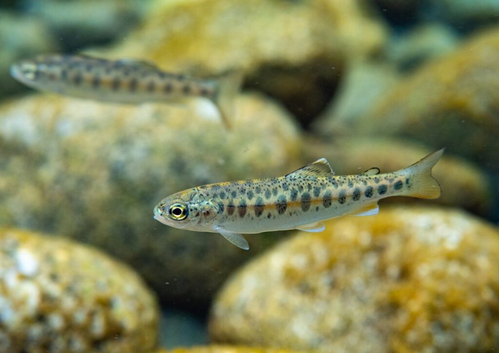
Image: Nick Chambers
Steelhead, as with most salmonids, don’t spawn evenly across a watershed. Some areas are used intensively, many areas are used by a few, and some areas are not used at all. So, what does the distribution of spawning adults have to do with fry?
More than you may think.
When females aggregate and spawn in close proximity, vast numbers of fry are forced to coexist in a small area for a few months, until the survivors eventually grow enough to successfully move further away from the redd and take advantage of other habitats with less competition.
When redds are less aggregated and are more spatially dispersed, lower densities lead to reduced competition.
Several studies have conducted research on redd distribution and its effect on fry growth and survival, all finding relatively similar results. One study constructed redds in two artificial stream channels in clustered and evenly spaced distributions (Einum 2008: Link). By the end of the summer, the stream sections with the evenly distributed redds had more and larger individuals than those with clustered distributions. This is because there was less competition for food and space when redds were not clustered. While this research was done on Atlantic Salmon, that species can be a good analog for steelhead. Their juveniles display similar territory sizes, likely due to both species spending several years in freshwater before smolting and migrating to the ocean.
Of course, some fry will move — sometimes substantial distances, up to 1,500m or so — to seek other habitat with less competition. Still, that movement comes at a cost, typically higher mortality, because moving several hundred meters as a small, vulnerable fish not only consumes precious energy, it also increases their likelihood of being preyed upon by fishes and other animals. Accordingly, most fry remain within 100-300m of the redd during the critical period.
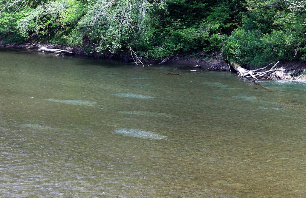
Image: John McMillan/TU
These findings have several implications. First, as with prior research, it indicates the period of greatest mortality occurs during the first few months of life, when up to 40-60% of the young fish may perish. It is important to know when mortality is highest in freshwater to understand and estimate a population’s potential for compensating with greater growth and survival.
Second, the distribution of redds influences growth and mortality of fry by increasing or decreasing density dependence. Consequently, when females aggregate and spawn in close proximity, vast numbers of fry are forced to coexist in a small area for a few months, until the survivors eventually grow enough to successfully move further away from the redd and take advantage of other habitats with less competition.
Third, because fry have a difficult time dispersing from the redd and because adults spawn unevenly throughout a watershed, the distribution and size of fry within a watershed is often closely related to the distribution and abundance of spawning adults. Habitat quality and quantity matters too, but, the strong relationship between the distribution of adults and fry is one reason that habitat alone is often a poor predictor of where fry are within a watershed (McMillan 2013: Link).
Taken together, the findings imply that relying solely on habitat, and not accounting for the early critical period in life, when mortality is greatest, and the distribution of adult redds may confound estimates of habitat capacity.
For instance, Finstad et al. (2013: Link) found escapement estimates that did not account for the distribution of redds and the limited dispersal of fry led to a downward bias in estimating escapement goals. More simply, adult spawners need to be thoroughly distributed throughout a watershed to account for the limited mobility of fry, and if the spatial distribution of spawners begins to contract, it can have carry-over effects that reduce productivity of the population. Not accounting for this could lead to escapement goals that are too low.
This has also been documented in steelhead. Atlas et al. (2015: Link) found that the productivity of Keogh River (British Columbia) steelhead declined as their distribution of spawners contracted, despite habitat quality and quantity remaining the same. This is a phenomenon known as depensation, which is the opposite of compensation. It is simply that as abundance decreases so does the productivity of a population. It is very difficult to identify the threshold where a population will switch from compensation to depensation and that is one reason it is critical to base management decisions on robust biological data.
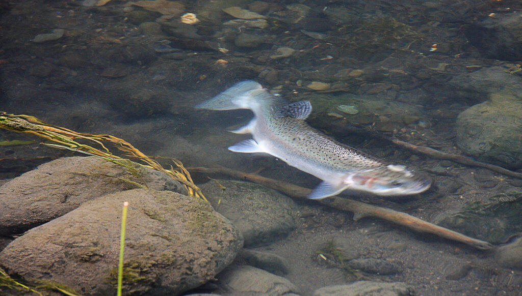
Image: John McMillan/TU
In summary, the distribution of spawning adults has important effects on density dependence and survival of fry, which needs to be accounted for when estimating escapement goals. While clustering of redds and breeding activity is normal, having too few fish in a system may impede the ability of fry to access all the available habitats if redds are not adequately distributed, effectively limiting their ability to compensate for lower densities. In situations where data on redd distribution and fry density dependence is scarce or lacking, assumptions based solely on habitat or density dependence at older life stages are therefore more likely to contribute to lower escapement goals.
This is critical. Salmon and steelhead today face large-scale changes in their freshwater and marine environments, leading to high levels of annual variation in survival rates. As we have seen this summer, with the very low runs in the Columbia, Skeena, North Umpqua, and other major steelhead-producing rivers, steelhead face an uncertain future. If we want a future with steelhead fishing, we need to make sure we are aligning management of their fisheries and habitat. One way to do that is to maximize the number of spawning fish, which will help increase and expand the distribution of spawners and fry in a given year. It will also improve odds that steelhead can compensate during the bad years.
Next week we look at how adults, juveniles, and density dependence are incorporated in stock-recruit models that are used to evaluate the capacity and productivity of steelhead and salmon populations. Until then, may the force of wild steelhead be with you all.


